A Guide for Multi-Label Classification

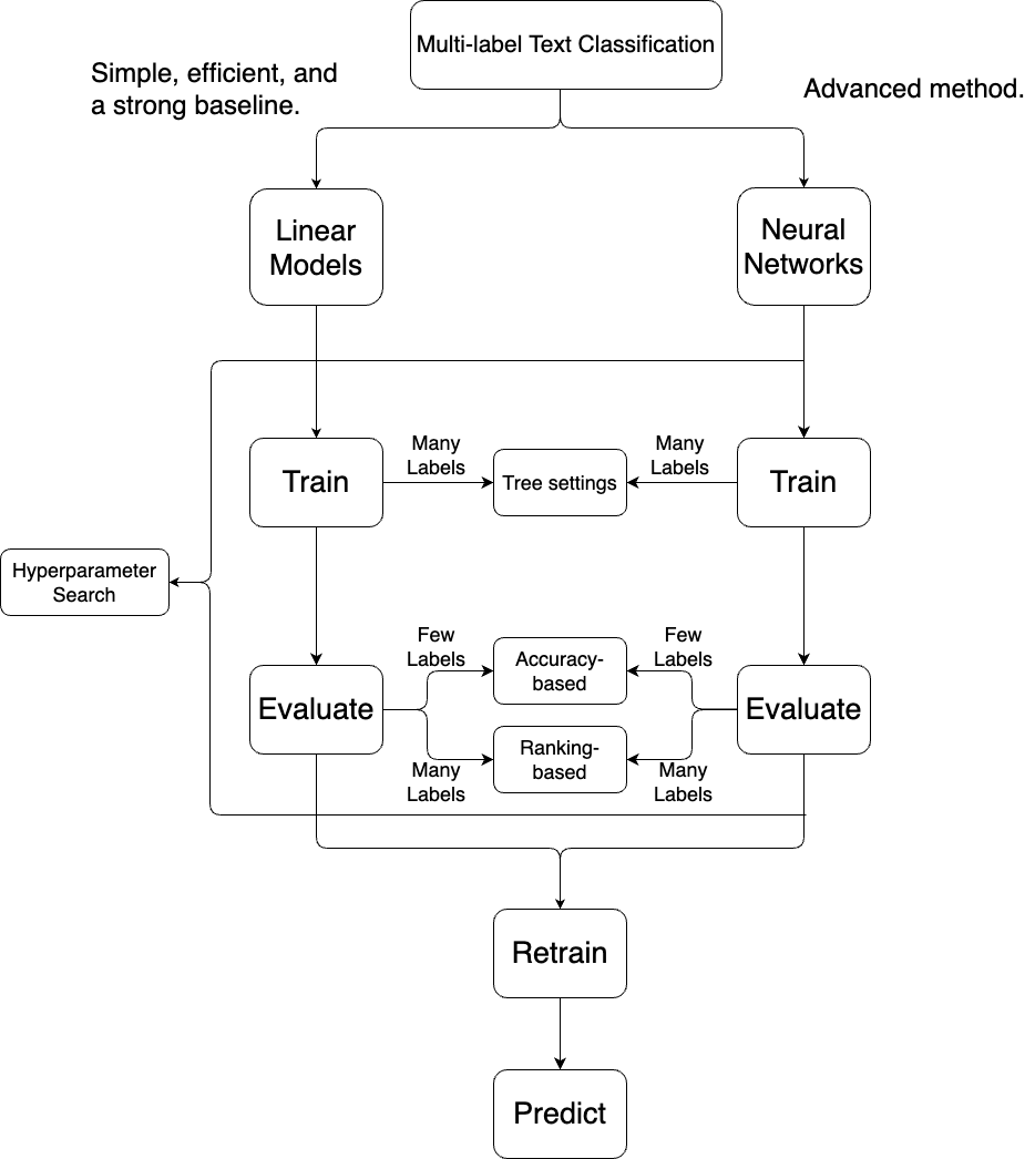
This tutorial serves as a high-level guide for multi-label classification. Users can follow the steps in this guide to select suitable training methods and evaluation metrics for their applications, gaining a better understanding of multi-label classification. Below is a flow chart summarizing this tutorial. We will explain each stage in the graph.

Depending on the number of labels in the application, multi-label classification requires different methods to achieve good efficiency and performance. To simulate different numbers of labels for users’ possible applications, this guide utilizes two datasets: one with a smaller label space, rcv1 (101 labels), and the other with a larger label space, EUR-Lex-57K (4,271 labels).

Details of the training methods and the evaluation metrics mentioned in this guide can be found in the implementation document.

Step 1. Linear Methods or Neural Networks

LibMultiLabel offers both deep learning and linear methods. Linear methods usually serve as strong baselines with better efficiency in training the models, while deep learning methods achieve state-of-the-art results with less efficiency. For more details, refer to the paper [LCLL22].

To showcase the difference, we provide an example using the rcv1 dataset to compare the two methods. The following code uses the one-vs-rest linear method on rcv1. This method, also known as binary relevance, trains a binary classification model for each label on data with and without that label. Detailed explanation of the following code can be found in the linear quickstart.

import libmultilabel.linear as linear
import time

datasets_rcv1 = linear.load_dataset("txt", "data/rcv1/train.txt", "data/rcv1/test.txt")
preprocessor_rcv1 = linear.Preprocessor()
preprocessor_rcv1.fit(datasets_rcv1)
datasets_rcv1 = preprocessor_rcv1.transform(datasets_rcv1)

start = time.time()
model = linear.train_1vsrest(datasets_rcv1["train"]["y"], datasets_rcv1["train"]["x"], "")
end = time.time()

preds = linear.predict_values(model, datasets_rcv1["test"]["x"])
target = datasets_rcv1["test"]["y"].toarray()
metrics = linear.compute_metrics(preds, target, monitor_metrics=["Macro-F1"])
print({"Macro-F1":metrics["Macro-F1"], "Training_time":end - start})

As the label space of rcv1 is small, we consider an accuracy-based metric Macro-F1; see Step 3 for more details.

The performance and training time are as follows:

{'Macro-F1': 0.5171960144875225, 'Training_time': 4.327306747436523}

For deep learning, we train a BERT model for this dataset. We exclude the code here for simplicity. Please refer to the BERT quickstart for details. Following the quickstart, the resulting performance and training time are as follows:

{'Macro-F1': 0.564618763137536, 'Training_time': 5412.955321788788}

The table below illustrates the performance and efficiency trade-off between these methods. Users can use this information to decide which method to employ depending on their specific application needs.

Methods	Macro-F1	Training time (sec)
Linear method (one-vs-rest)	0.52	4.33
Deep learning method (BERT)	0.56	5412.96

Step 2. Training:

If number of labels is small

Due to the nature of multi-label problems, there are often many more instances without a particular label than with it. As we mentioned, the one-vs-rest method trains a binary classifier for each label. When using this method, each binary problem becomes imbalanced, and the model will rarely predict some labels. This imbalance leads to unsatisfactory results when accuracy-based metrics like Macro-F1 are used (refer to Step 3 for the reason why Macro-F1 is often used when the number of labels is small). Some techniques can solve this problem, including thresholding and cost-sensitive methods. Because this is a high-level guide, we leave the details of data imbalance and the solutions in the implementation document. Below is an example of thresholding and cost-sensitive methods on rcv1 dataset.

model_threshold = linear.train_thresholding(datasets_rcv1["train"]["y"], datasets_rcv1["train"]["x"], "")

model_cost_sensitive = linear.train_cost_sensitive(datasets_rcv1["train"]["y"], datasets_rcv1["train"]["x"], "")

preds_threshold = linear.predict_values(model_threshold, datasets_rcv1["test"]["x"])
preds_cost_sensitive = linear.predict_values(model_cost_sensitive, datasets_rcv1["test"]["x"])

metrics_threshold = linear.compute_metrics(preds_threshold, target, monitor_metrics=["Macro-F1"])
metrics_cost_sensitive = linear.compute_metrics(preds_cost_sensitive, target, monitor_metrics=["Macro-F1"])

print({"Macro-F1":metrics_threshold["Macro-F1"]})
print({"Macro-F1":metrics_cost_sensitive["Macro-F1"]})

The performance of thresholding:

{'Macro-F1': 0.5643407144065415}

The performance of cost-sensitive:

{'Macro-F1': 0.5704056980791481}

Compare with the naive one-vs-rest method in Step 1:

Methods	Macro-F1
One-vs-rest	0.52
Thresholding	0.56
Cost-sensitive	0.57

From the comparison, one can see that these techniques improves the naive method.

As for the situation for deep learning, we are still investigating the problem and working on the solution.

If number of labels is large

When the label space is large, the imbalance problem is less of a concern because we only consider top predictions (refer to Step 3 for explanation). The challenge, however, shifts to efficiency in training the model. Training models directly in this case may result in high runtime and space consumption. A solution to reduce these costs is to utilize tree-based models. Here we provide an example comparing a linear one-vs-rest model and a tree model on the EUR-Lex-57k dataset, which has a larger label space. We start by training a tree model following the linear tree tutorial.

datasets_eurlex = linear.load_dataset("txt", "data/eurlex57k/train.txt", "data/eurlex57k/test.txt")
preprocessor_eurlex = linear.Preprocessor()
datasets_eurlex = preprocessor_eurlex.fit_transform(datasets_eurlex)

start = time.time()
tree_model = linear.train_tree(datasets_eurlex["train"]["y"], datasets_eurlex["train"]["x"])
end = time.time()

tree_preds = linear.predict_values(tree_model, datasets_eurlex["test"]["x"])
target = datasets_eurlex["test"]["y"].toarray()
tree_score = linear.compute_metrics(tree_preds, target, ["P@5"])
print({"P@5":tree_score["P@5"], "Training_time":end - start})

Different from Step 1, the label space of EUR-Lex-57k is large, so we use a ranking-based metric precision@5 here. Refer to Step 3 for more details.

In this case, the performance and training time of the tree model is:

{'P@5': 0.679, 'Training_time': 262.8317949771881}

If we follow the training procedure from Step 1 and train a one-vs-rest model, the performance and training time on this larger dataset will be as follows:

{"P@5": 0.6866666666666666, "Training_time": 1403.1347591876984}

It is clear that the tree model significantly improves efficiency. As for deep learning, a similar improvement in efficiency can be observed. Details for the tree-based deep learning model can be found in the deep learning tree tutorial.

Step 3. Evaluation: Pick Suitable Metrics

As for the evaluation of the model, the choice of the evaluation metric also depends on the application and the number of labels.

Consider problems with a small label space. In such cases, the goal is often to accurately predict every label relevant to an instance, making accuracy-based metrics appropriate choices. Accuracy-based metrics include Macro and Micro-F1.

In problems where there are thousands or even millions of labels, it is extremely difficult to exactly identify the label set of an instance from the vast label space. Furthermore, the goal of such applications is often to ensure that the top predictions are relevant to the user. In these cases, instead of metrics that consider the whole label set, like Macro-F1 and Micro-F1, ranking-based metrics such as precision at K (P@K) and normalized discounted cumulative gain at K (NDCG@K) will be more suitable.

For linear models, the evaluation metrics can be easily specified with the argument monitor_metrics in the compute_metrics function.

In Step 2, we mentioned that a ranking-based metric (precision@5) is used because the label space of the dataset (EUR-Lex-57k) is large. If we instead use Macro-F1 in Step 2, by the following code:

tree_score = linear.compute_metrics(tree_preds, target, ["Macro-F1"])
print({"Macro-F1":tree_score["Macro-F1"]})

the result will look like:

{'Macro-F1': 0.06455166396222473}

The Macro-F1 score for this dataset with more labels is close to zero, making this result not very informative.

For deep learning usage, please refer to the two quickstarts (BERT quickstart, CNN quickstart) for more details.

Step 4. Hyperparameter Search

Models with suboptimal hyperparameters may lead to poor performance [LYCL21]. Users can incorporate hyperparameter tuning into the training process. Because this functionality is more complex and cannot be adequately demonstrated within a code snippet, please refer to these two tutorials for more details about hyperparameter tuning (linear and deep learning). Another thing to consider is that hyperparameter search can be time-consuming, especially in the case of deep learning. Users need to conduct this step with consideration of the available resources and time.

Step 5. Retraining

The common practice in machine learning for hyperparameter search involves splitting the available data into training and validation sets. To use as much information as possible, for linear methods, after determining the best hyperparameters, all available data are generally trained under these optimal hyperparameters to obtain the final model. We refer to this as the “retrain” strategy.

For linear methods, the tutorial for hyperparameter search already handles retraining by default. As for deep learning, since this additional step is not common in practice, we include it in the last section of this tutorial.

Step 6. Prediction

In Step 1 and 2, we simply use the decision values from the model to compute the metrics. To get predicted labels of each test instance, users can use the following code (using the linear one-vs-rest model in Step 1):

pred_labels, pred_scores = linear.get_positive_labels(preds, preprocessor_rcv1.label_mapping)
prediction = []
for label, score in zip(pred_labels, pred_scores):
    prediction.append([f"{i}:{s:.4}" for i, s in zip(label, score)])
print(prediction[0])

The prediction for the first test instance will look like:

['GCAT:1.345', 'GSPO:1.519']

As for deep learning, please refer to the two quickstarts (BERT quickstart, CNN quickstart) for more details.