radial basis function network
The radial basis function network (RBFN) is a special type of neural networks
with several distinctive features
[Park and Sandberg, 1991,Poggio and Girosi, 1989,Ghosh and Nag, 2000,Mitchell, 1997,Orr, 1996,Kecman, 2001].
Since its first proposal, the RBFN has attracted a high degree of interest in
research communities. An RBFN consists of three layers, namely the input
layer, the hidden layer, and the output layer. The input layer broadcasts the
coordinates of the input vector to each of the nodes in the hidden layer. Each
node in the hidden layer then produces an activation based on the associated
radial basis function. Finally, each node in the output layer computes a
linear combination of the activations of the hidden nodes. How an RBFN reacts
to a given input stimulus is completely determined by the activation functions
associated with the hidden nodes and the weights associated with the links
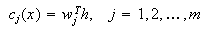
between the hidden layer and the output layer. The general mathematical form
of the output nodes in an RBFN is as follows:
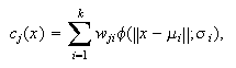 where
where
 is the function corresponding to the
 -
- output unit
(class-
output unit
(class- )
and is a linear combination of
)
and is a linear combination of
 radial basis functions
 with center
 and bandwidth
 .
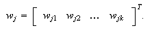
Also,
.
Also,
 is the weight vector of
class-
is the weight vector of
class- and
and
 is the weight corresponding to the
 -
- class
and
class
and
 -
- center. The general architecture of RBFN is shown as follows.
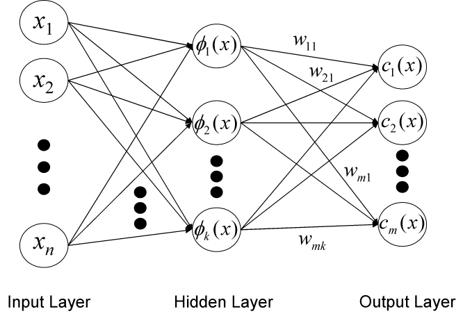
General Architecture of Radial Basis Function Networks
We can see that constructing an RBFN
involves determining the number of centers,
 ,
the center locations,
,
the center locations,
 ,
the bandwidth of each center,
,
the bandwidth of each center,
 ,
and the weights,
,
and the weights,
 .
That is, training an RBFN involves determining the values of three sets of
parameters: the centers
(
.
That is, training an RBFN involves determining the values of three sets of
parameters: the centers
( ),
the bandwidths
(
),
the bandwidths
( ),
and the weights
(
),
and the weights
( ),
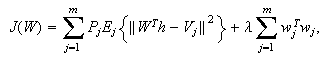
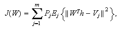
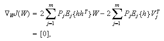
in order to minimize a suitable cost function.
),
in order to minimize a suitable cost function.


![$[0]$](graphics/icml05-1__81.png)