Q-learning Demo ( Solve the Inverted Pendulum Problem )
Here we write a demo program with GUI. You can download it with the link below
Install steps:
1. Download the file above.
2. Unzip it into the directory you like.
3. Execute the <Q_demo.exe> in win32 OS.
The GUI is showed below :
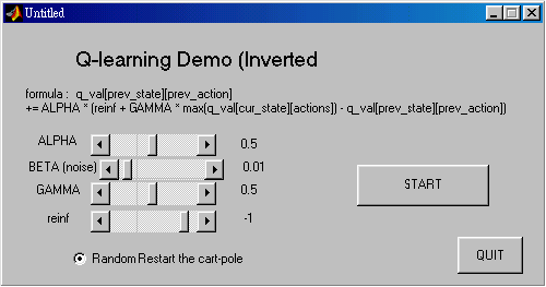
< Here you can set factors in equation below >
After you click the start button , you can see two windows bump out :
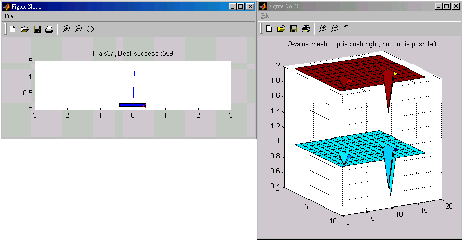
If you want to stop the current simulation, just close <Figure No.1> and <Figure No.2> window.
Q-learning with Look-up Table and Recurrent Neural Networks as a Controller for the Inverted Pendulum Problem
ABSTRACT
In reinforcement learning, Q-learning can discover the optimal policy. This paper discusses the inverted pendulum problem using Q-learning as controller agent. Two methods for Q-learning are discussed here. One is look-up table, and the other is approximation with recurrent neural networks.
1. INTRODUCTION
Q-learning is an incremental dynamic programming procedure that determines the optimal policy in a step-by-step manner. It is an on-line procedure for learning the optimal policy through experience gained solely on the basis of samples of the form:
(1.1)
where n denotes discrete time, and each sample
consists of a four-tuple described by a trial action an on state in that results in a transition to state jn=in+1 (in denote state at time n) at a cost
. And it is highly suited for solving Markovian decision problems without explicit knowledge of the transition probabilities. The requirement of using Q-learning successfully is based on the assumption that the state of the environment is fully observable, which in turn means that the environment is a fully observable Markov chain. However, if the state of the environment is partially observable, for example : the sensor device on the inverted pendulum may be imprecise, special methods are required for discovering the optimal policy. To overcome this problem, a utilization of recurrent neural networks combined with Q-learning as a learning agent had been proposed.
According to Bellman’s optimality criterion combined with value iteration algorithm, the small step-size version formula of Q-learning is described by
for all (i,a) (1.2)
where η is a small learning-rate parameter that lies in the range 0<η<1. And the other symbols are defined as : “ i ” is sate at time n; “ j “ is state at time n+1; “a” is the action been taken at time n; “
” is the transition probability defined as
; “
” is the cost as i, a, j are defined previously; “γ” is discount factor. By adjustingγ we are able to control the extent to which the learning system is concerned with long-term versus short-term consequences of its own actions. In the limit, when γ= 0 the system is myopic in the sense that it is only concerned with immediate consequences of its action. Asγ approaches 1, future costs become more important in determining optimal actions. Therefore we usually confine the discount factor 0<γ<1.
We may eliminate the need for this prior knowledge by formulating a stochastic version of Eq.(1.2) . Specifically, the averaging performed in an iteration of Eq. (12.37) over all possible states is replaced by a single sample, there by resulting in the following update for the Q-factor:
is the learning rate parameter at time step n for the state-action pair (i,a).
2. THE INVERTED PEDULUM PROBLEM
The inverted pendulum problem consists of a pole that is freely hinged on top of a wheeled cart, which can move on a one dimensional track of fixed length (Fig.1). The goal is to apply a fixed magnitude force to one side of the cart to accelerate it at each time step, so as to keep the pole always upright and within a fixed angle from the vertical, and to keep the cart away from the ends of the track.
Figure 1 : Inverted pendulum problem.
2.1 Dynamics of the Problem
The target system is characterized by four variables; the angle of the pole and its angular velocity
, and the horizontal position and velocity of the cart
. The equations governing the behavior of the system are given below:
(2.1) (2.2)
where ![]() (1.1kg) is the mass of
the cart plus the pole,
(1.1kg) is the mass of
the cart plus the pole, ![]() is the
gravity acceleration constant (9.8m/s2),
is the
gravity acceleration constant (9.8m/s2), ![]() is half the length of the pole(0.5m),
is half the length of the pole(0.5m), ![]() is the mass of the pole(0.1kg) ,
is the mass of the pole(0.1kg) , ![]() is the output of the agent (+10N or –10N),
is the output of the agent (+10N or –10N), ![]() denotes angular acceleration,
denotes angular acceleration, ![]() denotes horizontal acceleration. The pole must be kept within
denotes horizontal acceleration. The pole must be kept within ![]() from vertical, and the cart must be kept within
from vertical, and the cart must be kept within ![]() from the center of the track. This system is simulated numerically by Euler
method with a sampling period of
from the center of the track. This system is simulated numerically by Euler
method with a sampling period of ![]() =0.02s.
The angular and horizontal velocity formula are given below:
=0.02s.
The angular and horizontal velocity formula are given below:
 (2.2)
(2.2)
The angel and the horizon offset is updated according to :
 (2.3)
(2.3)
3 Q-LEARNING WITH LOOK-UP TABLE METHOD
This method is to build a table for saving Q-factor. It is suitable for small size problems. In this problem, the storage size depends on the state and the action amounts. The action size is just two : push left and push right. And we define the cart-pole system in to 162 states :
|
Cart position |
-2.4 ~ -0.8 |
-0.8 ~ 0.8 |
0.8 ~ 2.4 |
|
State |
1 |
2 |
3 |
|
Velocity of cart |
<-0.5 |
-0.5 ~ 0.5 |
>0.5 |
|
State |
1 |
2 |
3 |
|
Pole angle |
<-6 |
-6 ~ -1 |
-1 ~ 0 |
0 ~ 1 |
1 ~ 6 |
>6 |
|
State |
1 |
2 |
3 |
4 |
5 |
6 |
|
Angle velocity of the pole |
<-50 |
-50 ~ 50 |
>50 |
|
State |
1 |
2 |
3 |
Table 1. each variable’s state definition
Therefore, there are 3*3*6*3=162 states. The Q-factor table is somewhat like:
|
State |
Action: push left |
Action: push right |
|
1 |
-0.011231 |
-0.2533 |
|
2 |
-0.00655 |
-0.0354 |
|
* |
* |
* |
|
162 |
-0.20015 |
-0.005014 |
Table 2. Q-factor table
3.1 Learning procedure for this method
Algorithm:
1.Set Q-factor table all entries zero.
2.Initial cart and pole.
3.Get current state.
4.Determine a action according to equation : ![]() .
.
(action= { left, right} )
5.Push cart and get current state.
6.if fail, reinforcement = -1 and reset cart. Else reinforcement = 0.
7.Update Q according to equation :
(3.1)
8.Repeat 3-7, until the agent learns it.
The agent receive reinforcement from the world, and return an action to the world round and round as shown below:
Fig 2. Structure of the learning agent
4. SIMULATION
A test was considered successful if the agent could balance the pole for 1000000 successive iterations (about 5.56 hours in real time).
4.1 Simulation with Fixed Restart
The inverted pendulum task was simulated with the agent described before having the following parameters: learning rate η=0.2, discount factor γ=0.85. In the initial test, fixed restarts were used after the pole fell over. In this case, the agent took around 186 trials to succeed in the task (Fig.3).
Fig 3. Learning profile for fixed restart
Here set the restarts at
. The learning parameter η and discount factor γ are important factors for the agent to learn. In fact it is very hard to find the combination of η and γ so that the agent can learn to control the cart successfully. Most of it would stop making progress at 100~800 iterations. It needs some luck to succeed.
4.2 . Simulation with Random Restart
To enhance exploration, random restarts were used. The result is shown in Fig.4. In this case, the agent took around 146 trials to succeed in the task, with the parameters: learning rate η=0.5, discount factor γ=0.85.
Fig.4. Learning profile for random restart
Here set the restarts at ![]() ,
where –0.01<random<0.01. Random restart enhances exploration so that the
agent will become much easier to be trained. And it is clearly that it needs
less time to learn successfully. Below list possible
combinations of learning parameter η
and discount factor γ:
,
where –0.01<random<0.01. Random restart enhances exploration so that the
agent will become much easier to be trained. And it is clearly that it needs
less time to learn successfully. Below list possible
combinations of learning parameter η
and discount factor γ:
|
η γ |
0.1 |
0.2 |
0.3 |
0.4 |
0.5 |
0.6 |
0.7 |
0.8 |
0.9 |
|
0.1 |
|
|
|
|
|
870 |
198 |
|
|
|
0.2 |
|
|
|
|
|
352 |
6831 |
53 |
541 |
|
0.3 |
|
|
|
|
|
|
155 |
231 |
3225 |
|
0.4 |
|
|
|
|
|
|
|
283 |
1288 |
|
0.5 |
|
|
|
|
|
|
1383 |
|
590 |
|
0.6 |
|
|
|
|
|
|
|
|
|
|
0.7 |
|
|
|
|
|
|
|
120 |
|
|
0.8 |
|
|
|
|
|
|
|
|
|
|
0.9 |
|
|
|
|
|
|
|
|
|
Table 3. The trials needed for learning successfully
We can see the learning rate should be less than 0.5, and the discount factor should be lager than 0.5
The trajectory of the behavior of the agent after learning shows how the agent control the cart so that the pole is balanced at –0.21<angle<0.21 and the cart is restrained between –2.4m<position<2.4m.
Fig 5. Trajectory of the Pole angle – Pole angle velocity
Fig 6. Trajectory of the Cart position – Cart velocity
Fig 7. Trajectory of the Cart position – pole angle
5. Q-LEARNING FOR RECURRENT NEURAL NETWORKS
Although look-up table method is easy to implement, it needs large space for storing Q-factor. This paper discusses another way to store Q-factor, which is to use recurrent neural networks for getting Q-factor.
5.1 Structure of the Learning Agent
The learning agent’s main part is a recurrent neural network of the type which can produce outputs from its inputs immediately. The network is trained to output Q-values for the current input and the current internal state of the recurrent neural network. The output units of the network have a linear activation function to be able to produce Q-values of arbitrary magnitude. For the hidden units, the sigmoid function is used.
One of the output s of the network is selected by the equation:
(5.1)
if ![]() >
>![]() ,
push left. Else push right. The action selected is also fed back into the neural
network through a one step time delay (at-1), as well as the current
input from the environment yt , and the internal feedback.
,
push left. Else push right. The action selected is also fed back into the neural
network through a one step time delay (at-1), as well as the current
input from the environment yt , and the internal feedback.
Fig 8. Structure of the learning agent of recurrent neural network
5.2. Learning procedure for this method
Algorithm:
1.Initialize the neural network.
2.Initial cart and pole.
3. Get current state.
4. Obtain
for each action by substituting current state and action into the neural network.
5.Determine a action according to equation : ![]() .
.
(action= { left, right} )
6.Push cart and get current state.
7.if fail, reinforcement = -1 and reset cart. Else reinforcement = 0.
8.Generate ![]() according to
equation :
according to
equation :
(5.2)
use
to train the network as Fig9. shown.
8.Repeat 3-7, until the agent learns it.
Fig 9. Neural network layout for approximating the target Q-factor
5.2 Recurrent Neural Network Architecture, and Learning Algorithm
Here we use Elman network, which is similar to a three layer feed forward neural network, but it has feedback from the hidden unit outputs, back to its input.
Fig 10. Elman network which activations are copied from hidden layer to context layer on a one-for-one basis, with fixed weight of 1.0. Solid lines represent trainable connections.
Here use 14 neurons in hidden layer, and 1 neuron in output unit, and 163 neurons in input layer, which 162 neurons for 162 states and 1 neuron for action. The output units of the network have a linear activation function to be able to produce Q-values of arbitrary magnitude. For the hidden units, the sigmoid function is used. In this study, we used the error back propagation algorithm to train Elman network. BP does not treat the recurrent connections properly, but require little computation.
6. SIMULATION
I have to say sorry about the implementation of Q-learning for Elman network. Many ways are tried but failed to solve it. The best record of the agent is to keep the pole in 88 seconds. Probably the learning rate η and discount factor γ are critical to the learning procedure, but I cannot find good value of them.
But if we use loop-up table training result to train the neural network, the neural network can learn it.
7. SPACE REQUIREMENT (LOOK-UP TABLE VERSUS ELMAN NETWORK)
Neural network:
Number of inputs : 163
Number of hidden neurons : 14
Number of context neurons :14
Number of output neurons : 1
Number of biases : 14+1=15
Total number of synaptic weights and biases =
(163+14)*14 + 14*1 + 15 + 1 = 2058.
Look-up table:
Number of states : 162
Number of actions : 2
Size of table = 162*2 = 324
Although neural network method needs more space than look-up table in this problem, in large size problem it will require less space than look-up table.
References
[1] Ahmet Onat, “Q-learning with recurrent Neural Networks as a Controller for the Inverted Pendulum Problem”, The Fifth International Conference on Neural Information Processing, pp 837-840, October 21-23, 1998.
[2] Simon Haykin, “Neural Networks .second edition”, pp 603-631, 1998.
[3] Jeffrey L. Elman , “ Finding Structure in Time”, Cognitive Science 14, 179-211, pp 179-211, 1990.
Attachments:
1. Q-learning with Look-up Table in C code … Qlearning_table.cpp
2. Q-learning with Elman network in C code … Qlearning_elman.cpp
3. Demo of Q-learning with Look-up Table in matlab code … Q_learning_demo folder, see disk.